Keeping an Excel dashboard alive means making sure every chart, pivot table, and KPI reflects the latest numbers without manual rework. If you want to automate data updates in Excel, you need three tools working together: source data in table format, pivot table refresh options, and a small macro that does the clicking for you. This is for anyone building reports who hates updating the same dashboard twice.
Why does your source data need to be in table format?
The whole automation chain breaks if your raw data is just a plain range. Formatting your source as an Excel table is what lets new rows flow into pivots and dashboards automatically.
You can confirm it the same way shown in the file: select your data and check that the Table Design tab appears at the top. Once your information lives inside a table, pasting new rows below extends the range instantly, and every pivot connected to it inherits those rows the moment you refresh.
What happens if my data is not in a table? Pivot tables will only see the original range, so new rows get ignored even after refreshing. You would need to redefine the source manually every time.
How do I refresh pivot tables when new data arrives?
Once the new month's information is pasted into your source table, you have three ways to push that change into your pivots and dashboard.
Manual refresh with one click or a shortcut
Click any pivot table, go to PivotTable Analyze, and use either Refresh or Refresh All. The keyboard shortcut Alt + F5 does the same on the active pivot.
- Refresh updates only the selected pivot table.
- Refresh All updates every pivot connected to every source in the file.
- On heavy files, Refresh All can take longer, so use it when you really need everything in sync.
A single click is usually enough to see totals recalculate and the dashboard reflect the new data.
Auto refresh when opening the file
If you would rather not click anything, right click on a pivot, open PivotTable Options, go to the Data tab, and enable Refresh data when opening the file. From that point on, every time you close and reopen the workbook, pivots pull the latest numbers from the source.
Refresh automatically with a macro
This is the option that feels truly automated. A macro is a small piece of code that runs a repetitive task for you, in this case the refresh action, every time something changes in the sheet.
How do I write a macro to refresh a pivot table automatically?
Before writing anything, you need two names: the pivot table name and the worksheet name.
Go to PivotTable Analyze and rename your pivot to something clean like Ventas (Sales). Then check the worksheet code name, which in the example is TD3, the name shown in parentheses inside the Visual Basic editor.
Now right click the sheet tab and choose View Code. In the Visual Basic window:
- Select the worksheet that contains the pivot, using the code name in parentheses.
- Change the left dropdown from General to Worksheet.
- Change the right dropdown to Activate.
- Paste this line inside the procedure:
vba
ActiveSheet.PivotTables("Ventas").PivotCache.Refresh
Close the editor and you are done. Every time the sheet detects a change and gets activated, the pivot refreshes by itself, no clicks needed.
What if I have 20 pivot tables? Copy and paste the same line for each one, changing only the pivot name in quotes, for example Ventas, Vendedores, Agentes. Same recipe, different names.
How do I save an Excel file with macros enabled?
A regular .xlsx file will not keep your macro. If you try to autosave, Excel warns you that autosave cannot complete because the file must be macro enabled.
Go to Save As and choose Excel Macro Enabled Workbook (.xlsm). From now on, when someone opens the file, Excel will ask for permission to enable macros, and once approved, the auto refresh will work as expected.
How do I optimize a dashboard so it does not get slow?
Dashboards usually carry background colors and styling that repeat across thousands of empty cells, eating memory and slowing the file. Limiting your working area fixes that.
- Click the first empty column to the right of your dashboard.
- Press Ctrl + Shift + Right Arrow to select all columns to the end.
- Right click and choose Hide.
- Repeat the same with Ctrl + Shift + Down Arrow for rows below your content.
The result is a cleaner canvas, a lighter file, and a dashboard that focuses the eye exactly where the data lives.
Which of these three refresh methods fits better with how you build your reports? Drop your case in the comments and tell me if you would go manual, on open, or full macro.