Cleaning the same messy file every month drains hours you could spend on analysis. With Power Query in Excel, you can record each cleanup step once and let Excel repeat the entire process every time new data arrives. This walkthrough shows you how to transform raw sales files into a ready to use table without touching a single formula.
Why use Power Query to clean repetitive files?
If you receive the same report every month with double row headers, full names you need to split, missing calculated columns, and rows marked not specified that you always delete, you already know the pain. Power Query turns that manual checklist into an automated recipe.
In the example, four yearly files exist (2017 to 2020), but only 2017 and 2018 are placed inside the working folder. The other two stay outside on purpose, so you can later see how the refresh picks them up automatically once you drop them in [00:55].
What is Power Query? It is an Excel tool that records every transformation you apply to your data as reusable steps. Next time the file changes, you just click Refresh and the whole cleanup runs again.
How do I combine and transform files from a folder?
Open Excel, go to Data, Get Data, From File, From Folder, and point it to the folder with your yearly files. When the preview window appears, the key choice is the dropdown at the bottom.
- Combine and Load: works only when files are already clean and just need to be stacked.
- Combine and Load To: same idea, with a destination chooser.
- Combine and Transform Data: the right pick when you need to clean headers, split text, add columns, or filter values [02:30].
After choosing Combine and Transform, pick a sample file (2017 in this case) and Power Query opens its editor with every applied step listed on the right panel. Think of those steps as a cooking recipe Excel will follow forever.
How do I fix two row headers with transpose and merge?
The first problem is the double header row. By default, Power Query promotes the first row as headers, so you delete that step using the X next to Promoted Headers.
Then go to Transform, click Transpose, and your columns become rows. Select the two columns that hold the split header text, right click, and choose Merge Columns. Pick a space as separator, name it Combined, and accept.
Now transpose again. The two header rows are fused into one. Click the small icon at the top left of the table and choose Use First Row as Headers. The cabeceras issue is solved permanently [05:10].
How do I extract a first name and split a delimited field?
To keep only the first name from a long Name Apellido Apellido string, select the column, go to Add Column, and pick Column From Examples. Type Robert in the first row, press Enter, and Power Query infers the pattern for every row. Rename the new column Name.
When should I use Transform vs Add Column in Power Query? Use Transform when you want to edit the existing column. Use Add Column when you want to create a new column based on a calculation or extraction, keeping the original intact.
For the Shipping Mode Container field separated by space dash space, select the column, go to Transform, Split Column, By Delimiter, choose Custom, and type the exact pattern. Two clean columns appear, which you rename to Shipping Mode and Container [07:40].
How do I add calculated columns and a date difference?
To build the Sales Amount column, select Quantity and Unit Price holding Ctrl, go to Add Column, Standard, and click Multiply. Rename the result Sales Amount.
For the delivery time, the selection order matters. Click Delivery Date first, then Ctrl click Order Date. Power Query grays out options that do not apply and keeps Date active. Choose Subtract Days and rename the column Delivery Days [09:30].
Finally, filter out rows where the value reads not specified. Click the column filter, uncheck that value, and accept. From now on, those rows will never appear again.
How do I detect data types and load the final table?
Before loading, select all columns with Shift and go to Transform, Detect Data Type. The ABC123 icon on each header tells you the current format. After detection, review every column: text, whole number, decimal, date, percentage.
If the discount column comes as a plain number but represents a percentage, click the icon and switch to Percentage. Power Query asks whether to replace the current step or add a new one; replacing keeps the steps clean.
- Go to Home, Close and Load To.
- Choose Table as the output.
- Confirm and let Excel populate the sheet.
When the 2019 and 2020 files land in the same folder, just hit Refresh and every transformation runs on the new data. That is the real payoff: you cleaned the file once, and your future self will never repeat those clicks.
Which of these steps would save you the most time in your weekly reports? Drop your scenario in the comments and let's troubleshoot it together.