Matrices are not just containers of numbers. They are dynamic operators that can stretch, rotate, or tilt any vector in space. Understanding linear transformations is the bridge between abstract algebra and real applications like computer graphics, robotics, and machine learning, and it is the key to unlocking what comes next in linear algebra.
What is a linear transformation and why does it matter?
A linear transformation is a function that takes an input vector and moves it to a new location, producing an output vector. But not every movement qualifies. To be linear, the transformation must satisfy two strict conditions that keep the geometry predictable.
- Parallel lines stay parallel and evenly spaced after the transformation. The grid can stretch or rotate, but it never curves.
- The origin stays fixed. In a 2D plane, the point (0,0) always maps to (0,0).
What makes a transformation linear? It preserves parallel lines with even spacing and keeps the origin fixed. If either rule breaks, the transformation is not linear.
Think of it like stretching a sheet of graph paper. You can pull it in any direction or twist it, but you cannot fold it or pinch it.
How do matrices encode space transformations?
Every 2x2 matrix tells you exactly where the standard basis vectors i-hat and j-hat land after the transformation. The first column is the new position of i-hat, and the second column is the new position of j-hat. That is the whole trick.
Scaling, rotation, and shear in action
Three classic examples make this idea concrete.
- Scaling matrix with values 2, 0, 0, 2. It doubles the size of the entire space. Every vector grows twice as long while keeping its direction.
- Rotation matrix with values 0, 1, -1, 0. It rotates the space 90 degrees counterclockwise. The yellow vector and the basis vectors all swing to the left.
- Shear matrix with values 1, 0, 1, 1. It tilts the space to the right. The vector i-hat stays put, but j-hat slides one unit to the right, slanting everything with it.
In every case, the columns of the matrix are exactly where i-hat and j-hat end up. That is why a matrix is essentially a recipe for moving the entire grid.
Why knowing where i-hat and j-hat go is enough
Here is the magic: if you know the new positions of i-hat and j-hat, you know where every other vector in the space lands. Any vector is just a combination of those two basis vectors, so once the basis moves, everything else follows along.
How do you apply a transformation with the matrix-vector product?
The operation is called the matrix-vector product, written as Ax or A·x, where A is the matrix and x is the vector. There are two ways to compute it, and both lead to the same answer.
Method 1: row by row
Let A be the shear matrix with values 1, 0, 1, 1, and let x be the vector 2, 1. Treat A as a stack of row vectors and apply the dot product to each row with x.
- First row (1, 1) · (2, 1) = 1·2 + 1·1 = 3.
- Second row (0, 1) · (2, 1) = 0·2 + 1·1 = 1.
The result is the vector 3, 1. The yellow input vector at (2,1) has been transformed into a new vector at (3,1), exactly where the shear matrix predicted it would land.
Method 2: linear combination of basis vectors
This approach is more elegant because it reveals the underlying logic. Since x = 2, 1 can be written as 2·i-hat + 1·j-hat, and since A sends i-hat to its first column (1, 0) and j-hat to its second column (1, 1), you can rewrite the product as:
Ax = 2·(1, 0) + 1·(1, 1) = (2, 0) + (1, 1) = (3, 1).
Same answer. But now you see clearly that the matrix-vector product is just a weighted sum of the columns of the matrix, with the weights coming from the input vector.
What is the matrix-vector product? It is the operation Ax that applies a linear transformation A to a vector x. You can compute it row by row with dot products or as a linear combination of the matrix columns.
Where do linear transformations show up in the real world?
Beyond the theory, linear transformations are the engine of computer graphics. Every time a character in a video game moves, jumps, or rotates, the game engine is applying a series of transformation matrices, such as rotations, translations, or scalings, to the vectors that define the character's position in the 3D world.
The same idea powers image filters, 3D modeling software, robotics arms, and the geometric layers of neural networks. If you can describe the motion as a matrix, you can compute it instantly.
Practice exercise to lock in the concept
Create a 2x2 matrix A with values 0, 1, 1, 0, and a vector x with values 3, 1. Apply the transformation to the vector and share a sketch of the original vector and the transformed one in the comments.
What does the matrix 0, 1, 1, 0 do? It swaps the x and y coordinates of any vector, reflecting the space across the diagonal line y = x.
If this concept still feels slippery, replay the class as many times as you need. Mastering matrices as transformations is the foundation for everything that comes next.