Recursos
Resumen
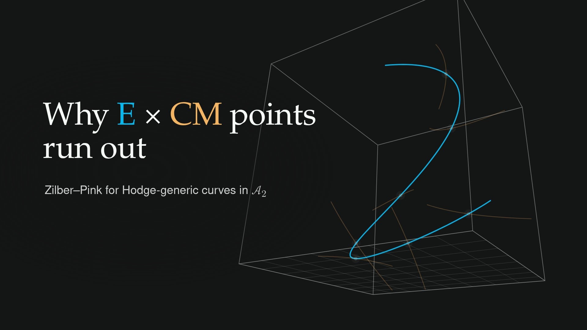
Take a Hodge-generic curve in A₂ and explain why it can hold only finitely many points whose abelian surface is isogenous to the square of a non-CM elliptic curve. You should also be able to say which theorem handles any special point on that curve.
The problem and the three branches
In the three-dimensional space A₂, a curve and a special curve have dimensions that add to 1 + 1, which is less than 3. So any meeting between them is unlikely. But special curves come in infinite families that include every Hecke translate [0:08]. At a point that is Hodge generic on a special curve, the surface falls into exactly one of three cases [0:53]:
- E × F, with E non-CM and F CM: handled by the companion theorem (A).
- E², with E non-CM: the paper's Theorem 1.1. The isogeny need not respect the polarization, so the condition is just End⁰(A_s) ≅ M₂(ℚ).
- An indefinite quaternion division algebra: handled by the companion theorem (B). It is division, so the split algebra M₂(ℚ) belongs to the E² branch [1:36].
These three finite sets, plus André–Oort for special points, give the full curve case of Zilber–Pink in A₂.
The chain behind Theorem 1.1
- Daw–Orr counting: if each elliptic-square point has a Galois orbit of size at least cΔ^δ, the locus is finite. Here Δ is the discriminant of the full endomorphism order [2:10].
- Two estimates [2:37]: the new height bound h ≤ c d^κ, and Masser–Wüstholz, Δ ≤ c(dh)^κ′. Substituting one into the other gives Δ ≤ c d^{κ′(κ+1)}, so d ≥ cΔ^{1/(κ′(κ+1))} [2:55].
- Where the height bound comes from [3:30]: fix a center t₀. Cross pairings ⟨B, Y(a)P⟩ between the endomorphism planes become traces at good reduction. Frobenius conjugation gives ⟨B, Y(a)P⟩ = ⟨B′, Y′(aR)P′⟩, an equation with no residue characteristic in it. This leaves only polynomially many systems in d.
- Two prime levels [4:27]: at ℓ₁, a degenerate incidence rules out both signs of a hidden identity. At ℓ₂, a nondegenerate incidence excludes nearby targets at places where the center has bad reduction.
- Interpolation with graph descent [5:13]: either the height is bounded or the dimension drops. The graph saves one power of L, which gives h ≤ C d^C.
Using it in your own reading
When a paper claims finiteness for a special-curve locus, first find the orbit bound in the complexity. Then find the height bound that feeds it, and check what that height bound assumes [5:50]. This proof needs no boundary degeneration and no bound on the number of proximity primes.